Last time we saw that we could come close to generating a curve that closely matches that of the differential of our state of charge curve.
As mentioned then, the differential defines the instantaneous rate of change at any point on the curve. We improved our estimate by making the difference between the points we were using to estimate the rate of change curve smaller. In the case of the differential, that differnce is considered infinitetismal.
In mathematics, an infinitesimal number is a non-zero quantity that is closer to 0 than any non-zero real number is.
Infinitesimal, on Wikipedia
So, it would seem to make sense, that if we keep reducing the gap between the two points used to estimate the differential, we should get closer to the actual value for the differential at any point in time. We will pursue that idea. Hopefully producing a function who’s output matches that of the differential function to some reasonable number of decimal places.
Graphical Interpretation of Differential
Before we get into building a function that estimates the differential for our battery state of charge curve, I think an attempt to picture what the differential actually is might be in order.
We will zoom in on ever tighter sections of the curve, plotting the rate of change for some portion of that small bit of curve. We will repeat that a few times until we meet a general criteria—to be explained as we go along. We will be using the brief discussion of the differential in the introduction above to quide us in this endeavour.
Convergence
Let’s look at the motivation for the criteria mentioned above.
Here’s some terminal output if I use a 19 item series of reducing time differences for calculating the rate of change for each time interval for specific time of day (16:00).
(mc-3.14) PS R:\learn\mc\calculus> python p_p1.py
i: 1: t1 - t2 = 15.5 - 16.5
rate of change: y = 4.698942919921862x + 0.9938278174899864
i: 2: t1 - t2 = 15.75 - 16.25
rate of change: y = 4.709025304570304x + 0.8325096631149194
... ...
i: 16: t1 - t2 = 15.999984741210938 - 16.000015258789062
rate of change: y = 4.712388980202377x + 0.7786908530017485
i: 17: t1 - t2 = 15.999992370605469 - 16.00000762939453
rate of change: y = 4.712388980202377x + 0.7786908530017485
i: 18: t1 - t2 = 15.999996185302734 - 16.000003814697266
rate of change: y = 4.712388977408409x + 0.778690897705232
i: 19: t1 - t2 = 15.999998092651367 - 16.000001907348633
rate of change: y = 4.71238898485899x + 0.7786907784959425
df/dhr(16) = 4.712388980384694
Priot to iteration 18 the rate of change is converging to some value. Starting at interation 18, the results cease to converge. Which means our estimated instantaneous rate of change is headed to who knows where. But most certainly not the value we are after.
New Rate of Change Function
I am going to create a new function, est_df()), which will for a given time estimate the differential at that point on the curve. It is somewhat based on the rate_chg() function. But, it has a few key differences. First, I will no longer be passing in a time delta value. Those values will be generated in the function and used in a loop to try and estimate a reasonable differential for the specified time. The specified time will be in the middle of each reducing time interval used to estimate the differential. And, I will be introducing a tolerance value to attempt to eliminate the problem described above. That tolerance value will be controlled by the n_dec parameter. I use the same parameter to determine how many time delta values to generate and loop over.
For document/debug purposes I added some print statements with a variable to control whether the print statements are excuted. Totally unnecessary for estimating the differential.
def est_df(fn, hr, n_dec=6):
  do_prn = True
  soc = fn(hr)
  tolr = 10 ** (-n_dec)
  prev_roc, _, _ = rate_chg(fn, hr-1, hr+1)
  t_zs = [2**(-i) for i in range(2, n_dec*2)]
  for i, t_z in enumerate(t_zs):
    if do_prn:
      print(f"i: {i+1}, t_z: {t_z}:", end="")
    t_spc = t_z / 10
    t_lw, t_hg = hr - t_z, hr + t_z
    t = np.arange(t_lw, t_hg+(t_spc / 2), t_spc)
    if do_prn:
      print(f", t2 - t12 = {t_hg} - {t_lw} = {t_hg - t_lw}")
    # s = fn(t)
    roc, _, _ = rate_chg(fn, t_lw, t_hg)
    if do_prn:
      # print(f"\t\tprev df: {prev_roc}, est df: {roc}")
      f_ln, y_int = mk_ln_fn(roc, hr, soc)
      print(f"\trate of change = {roc:.9f}x + {y_int:.9f}")
    if abs(prev_roc - roc) < tolr:
      # print(f"\tlast iter: {i+1} / {len(t_zs)}")
      return roc
    else:
      prev_roc = roc
  raise Exception("est differential did not converge!")
Let’s test the function.
if do_tngnt:
  # let's try to visualize what the differential represents
  t_hr = 16
  bc_hr = soc_fn(t_hr)
  d_hr = df_soc(t_hr)
  dgts = 9

  # print statments in function enabled
  e_dfhr = est_df(soc_fn, t_hr, n_dec=dgts)

  df_dhr, df_int = mk_ln_fn(d_hr, t_hr, bc_hr)
  print(f"df/dhr({t_hr}) = {d_hr:.9f}x + {df_int:.9f}")
(mc-3.14) PS R:\learn\mc\calculus> python p_p1.py
i: 1, t_z: 0.25:, t2 - t12 = 16.25 - 15.75 = 0.5
        rate of change = 4.709025305x + 0.832509663
i: 2, t_z: 0.125:, t2 - t12 = 16.125 - 15.875 = 0.25
        rate of change = 4.711547926x + 0.792147715
i: 3, t_z: 0.0625:, t2 - t12 = 16.0625 - 15.9375 = 0.125
        rate of change = 4.712178708x + 0.782055201
... ...
i: 11, t_z: 0.000244140625:, t2 - t12 = 16.000244140625 - 15.999755859375 = 0.00048828125
        rate of change = 4.712388977x + 0.778690901
i: 12, t_z: 0.0001220703125:, t2 - t12 = 16.0001220703125 - 15.9998779296875 = 0.000244140625
        rate of change = 4.712388980x + 0.778690863
i: 13, t_z: 6.103515625e-05:, t2 - t12 = 16.00006103515625 - 15.99993896484375 = 0.0001220703125
        rate of change = 4.712388980x + 0.778690853
df/dhr(16) = 4.712388980x + 0.778690850
And, that appears to have worked as desired.
Plots of Zoomed in Rates of Change
For a few of the points in the loop of time deltas, I generated a zoomed in plot of the curve and the line for the rate of change. Won’t bother with the code. Here’s four of those plots.
Note, Matplotlib’s use of a offset for the values on the x-axis for the last two plots.
The default formatter will use an offset to reduce the length of the ticklabels.
Frequently Asked Questions
Doesn’t look to me like they were reduced by all that much.
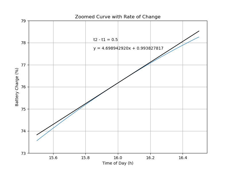
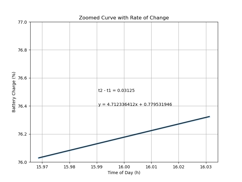
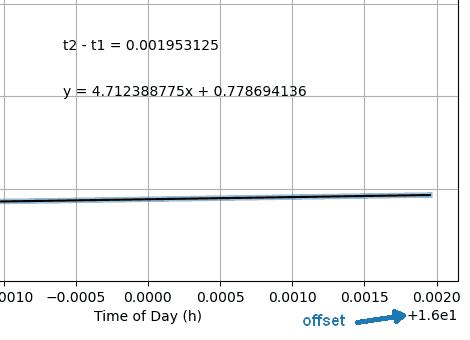
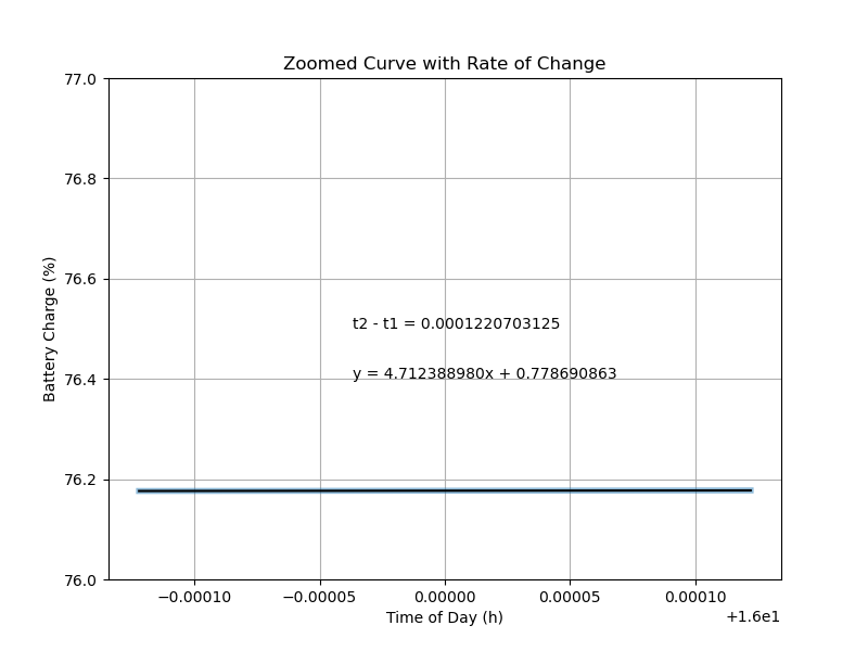
Pretty clearly, as the portion of the curve gets smaller and smaller, the rate of change line gets closer and closer to matching the curve. I.E. we are slowly converging on the instantaneous rate of change. On that last plot, my eyes don’t see any perceptible difference between the two.
Plot Line for Estimated Instantaneous Rate of Change
Okay, let’s plot the state of charge curve along with the line for the estimated differential at 16:00. Lot’s of plotting code last few posts, so just the plot.
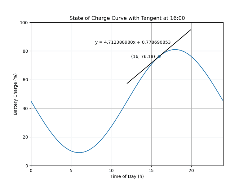
Now it may not be obvious but that line does not represent the slope of any portion of the curve. (Perhaps a little more obvious if we really zommed in on it.) That rate of change line in fact represents the tangent to the curve at 16:00 hours.
In geometry, the tangent line (or simply tangent) to a plane curve at a given point is, intuitively, the straight line that “just touches” the curve at that point. Leibniz defined it as the line through a pair of infinitely close points on the curve. More precisely, a straight line is tangent to the curve y = f(x) at a point x = c if the line passes through the point (c, f(c)) on the curve and has slope f’(c), where f’ is the derivative of f.
Tangent
Bit of a circular definition that one. But, it does explain the relationship of the differential (instantaneous rate of change) and the tangent we drew in the plot above.
Confirming Our Differential Function
Okay, before calling it a day, let’s look at plotting our function’s estimated differential for a series of points over the actual curve of the differential function. We’ve seen this before. So no code just the terminal output and the plot.
(m4p-3.14) PS R:\learn\m4p\calculus> python txt_loc.tst.py
1: tangent for est_df(0.0) = -9.424777959x + 45.0
2: tangent for est_df(1.0) = -9.103636438x + 44.78615081410345
3: tangent for est_df(2.0) = -8.162097138x + 43.324194275337504
4: tangent for est_df(3.0) = -6.664324406x + 39.537129095534254
5: tangent for est_df(4.0) = -4.712388977x + 32.672641372418866
6: tangent for est_df(5.0) = -2.439312030x + 22.423230405835994
7: tangent for est_df(6.0) = 0.000000000x + 8.999999999999998
8: tangent for est_df(7.0) = 2.439312030x + -6.848513959545899
9: tangent for est_df(8.0) = 4.712388977x + -23.876026353557112
10: tangent for est_df(9.0) = 6.664324406x + -40.43476377707273
11: tangent for est_df(10.0) = 8.162097138x + -54.62097137683304
12: tangent for est_df(11.0) = 9.103636438x + -64.45748644006717
13: tangent for est_df(12.0) = 9.424777959x + -68.09733550914098
14: tangent for est_df(13.0) = 9.103636438x + -64.02978806876882
15: tangent for est_df(14.0) = 8.162097138x + -51.26935992715881
16: tangent for est_df(15.0) = 6.664324406x + -29.509021970062108
17: tangent for est_df(16.0) = 4.712388977x + 0.7786909014305223
18: tangent for est_df(17.0) = 2.439312030x + 38.30502522884396
19: tangent for est_df(18.0) = 0.000000000x + 81.0
20: tangent for est_df(19.0) = -2.439312030x + 126.12025832485867
21: tangent for est_df(20.0) = -4.712388977x + 170.42469407975136
22: tangent for est_df(21.0) = -6.664324406x + 210.4066566513823
23: tangent for est_df(22.0) = -8.162097138x + 242.56613703351468
24: tangent for est_df(23.0) = -9.103636438x + 263.7011236916185
25: tangent for est_df(24.0) = -9.424777959x + 271.1946710217744
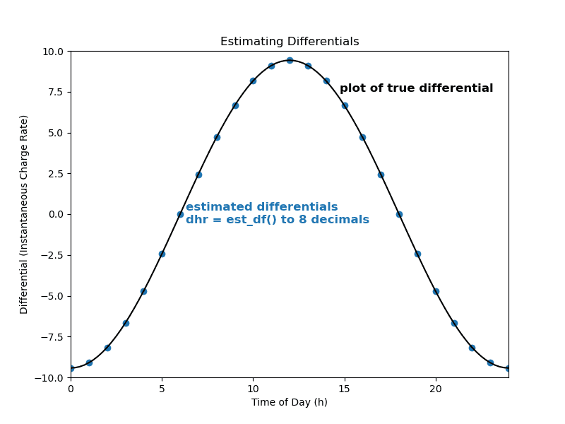
Pretty good fit, m’thinks.
Done
I think this post is finished. Over the last few posts, fairly good coverage of the differential without any mind-boggling theorems or proofs.
I did have something that bothered me when working on the plots at various stages of this discussion of the differential. I am not currently sure, but I may waste some time and a post trying to sort out my discomfort.
If not, I will move on to having a look at the differential’s best friend: integration.
Until next time, do enjoy playing around with math and coding.
Note
After writing the above, I realized I had failed to do/cover something I had planned to do/cover. I wanted to write a function that would generate the rate of change curve for the day. Will code/cover that when I get back to sorting calculus with geometry and code.
Resources
- Text in Matplotlib
- Prevent ticklabels from having an offset
- Matplotlib text dimensions
- How can I remove or change text from a matplotlib plot?