Well, my little side-trip, away from calculus, has certainly turned into a rollercoaster ride. One which is not quite yet done. Though, of course, that geometrical look at calculus is.
I believe the data point and text plotting is under control. With a new function to do all the work given the data point coordinates. Well, plus a few extra bits of information.
Drawing Tangents
Let’s move on to part two of the matplotlib and text battle: drawing the tangent line and labelling it with its equation. I am going to write one function that does both: line and text. At this point, I am not sure that it needs anything more, in the way of parameters, than what we are passing to the data point drawing function. But, I may, well almost certainly, look at a separate function to do some or all of the work for plotting the tangent. Separation of interests and all.
Core Function, Initial Design
Let’s start with an introductory look at the probable core tangent/text plotting function’s basic design. Note the calls to support functions—will code those next and perhaps change signatures. Best guess for now.
def draw_tangent_txt(ax, px1, py1, px2, slp, p_font):
  ''' Calculate the point at which to place tangent equation text.
      Plot tangent and draw text to supplied figure axis.

  :param ax: matplotlib plot axes
  :param px1: x-axis value for point of interest
  :param py1: y-axis value for point of interest
  :param px2: the inverse x value if it exists, i.e. closest x where fn(x) = ty1
  :param slp: differential for (tx1, ty1), i.e. slope of tangent line
  :param p_font: initial font dict to use for point related text
                 keys expected: 'color', 'size', 'va'
                 'color' and 'size' values will not change,
                 'ha' may be added, and 'va' changed

  :returns: nothing, plots tangent and draws related text to figure axis, ax.
  '''
  # we could use ax.get_window_extent to determine these values, but...
  # x_min, x_max = 0, 24
  # at this point should only be one Line2D object on the plot,
  #  the state of charge curve
  if len(ax.lines) == 1:
      x_min, x_max, y_min, y_max = get_artist_bbox(ax.lines[0])

  x_sep = .3
  is_ok = False
  t_font = copy.deepcopy(p_font)

  t_str, t_fn, t_inv, t_bbx = draw_tangent(ax, px1, py1, slp, p_font)

  # code to sort text position and draw text to passed axis
  # if tangent extents below or above soc curve put text between curve
  #   axis min/max as appropriate depending on where tangent line ends

  # otherwise put code ??

  # return anything?
get_artist_bbox()
Okay let’s start with the first supporting function. It is used in the function above and in the support function draw_tangent(). Perhaps elsewhere. The test code will be in a new if block, txt4.
We have seen this function’s code before. And, going to keep it simple. Had thought about sorting the bbp values in some way, but decided to not do so. At this point and for this function unnecessary work and code.
def get_artist_bbox(a_ln):
  ''' Return the min/max x/y values for passed in artist
  '''
  r = fig.canvas.get_renderer()
  bbp = a_ln.get_window_extent(renderer=r).transformed(plt.gca().transData.inverted())
  return bbp
Quick test on the underlying state of charge curve.
if blk_2b["txt4"]:

  # plot state of charge function
  fig, ax = plt.subplots(figsize=(8, 6))
  t = np.arange(0.0, 24.0, 0.05)
  s = soc_fn(t)
  xl = (0, 24)
  yl = (0, 100)
  socp = soc_plot(ax, t, s, xl, yl, params={"c": "k"})

  # ax.plot returns a list, should only be one entry in the list
  l_bbx = get_artist_bbox(ax.lines[0])
  print(l_bbx)
And, in the terminal, that code output the following.
(mc-3.14) PS R:\learn\mc\calculus> python txt_loc.py -c txt4
Bbox(x0=0.0, y0=8.999999999999998, x1=23.950000000000003, y1=81.00000000000001)
And, we know from past work that the x-axis goes from \(0 - 24\). And that, give or take, the curve minima is \(9\) and the maxima is \(81\).
draw_tangent()
Okay, let’s move on to some code a touch more complex. We will draw the tangent on the axis provided to the raw_tangent_txt() function. I expect that function is going to need a fair bit of information regarding that tangent line. So, for now, I have draw_tangent() calculating and returning the following information to the caller:
- tangent line equation in string form
- tangent line equation (function)
- tangent line inverse equation (function)
- tangent line bounding box
def draw_tangent(ax, px1, py1, slp, p_font):
  ''' Draw appropriate tangent line on provided plot axis
    then return data specific to tangent and line artist

  :param ax: plot axis
  :param px1: data point x-value
  :param py1: data point y-value
  :param slp: estimated differential at the given point
  :param p_font: font dict to use to draw tangent line

  :returns:
    - string verion of tangent line equation
    - function for tangent line equation
    - function for inverse of tangent line equation
    - tangent line bounding box
  '''
  ln_fn, y_int = mk_ln_fn(slp, px1, py1)
  ln_inv = lambda y: ((y - y_int) / slp)
  t_txt = f"y = {slp}x {'+' if y_int>=0 else '-'} {abs(y_int)}"
  # roughly plot to time range of (time -/+ 4 hours)
  t = np.arange(max(0, px1-4), min(24, px1+4), 0.05)
  p_l = ln_fn(t)
  a_ln = ax.plot(t, p_l, c="k")
  l_bbx = get_curve_bbox(a_ln[0])
  return t_txt, ln_fn, ln_inv, l_bbx
For this test we will need a data point on the state of charge curve and a figure showing the state of charge plot. We will draw the tangent at the chosen point against the state of charge curve. A fair bit more code than the test above. I am repeating the code from above.
if blk_2b["txt4"]:

  # plot state of charge function
  fig, ax = plt.subplots(figsize=(8, 6))
  t = np.arange(0.0, 24.0, 0.05)
  s = soc_fn(t)
  xl = (0, 24)
  yl = (0, 100)
  socp = soc_plot(ax, t, s, xl, yl, params={"c": "k"})

  l_bbx = get_artist_bbox(ax.lines[0])
  # print(l_bbx)

  px = 3.0
  px = 23.5
  px = 20.5
  py = soc_fn(px)
  p_df = est_df(soc_fn, px, n_dec=9)
  px2 = soc_inv(py, px)

  print(f"at ({px}, {py})")
  # plot point and related text
  p_font = {
    'color': 'b',
    'size': 9,
    'va': "center",
  }
  draw_dpt_txt(ax, px, py, px2, p_df, p_font)

  t_font = {
    'color': 'k',
    'size': 9,
    'va': "center",
  }
  # plot tangent -- test, will not actually use this function
  # will be called from draw_tangent_txt()
  t_str, t_eq, t_inv, t_bbx = draw_tangent(ax, px, py, p_df, t_font)
  print("\t", t_str, "\n\t", t_bbx)
  print(f"\tt_eq({px}): {t_eq(px)}")
  print(f"\tt_inv({py}): {t_inv(py)}")
  print(f"\tfor bbx.x1: t_eq({t_bbx.x1}): {t_inv(t_bbx.x1)}")

  i_blk = 0
  if blk_2b["sv_plt"]:
    fig.savefig(f"img/text_3_{i_blk + 1}.png")
  plt.show()
And in the terminal I got the following.
(mc-3.14) PS R:\learn\mc\calculus> python txt_loc.py -c txt4 -s
args: Namespace(code_block='txt4', item=None, save=True)
at (20.5, 73.56072025048448)
         y = -5.737441299133934x + 191.17826688273013
         Bbox(x0=16.5, y0=53.7665477684718, x1=23.950000000000102, y1=96.51048544702022)
        t_eq(20.5): 73.56072025048448
        t_inv(73.56072025048448): 20.5
        for bbx.x1: t_eq(23.950000000000102): 53.76654776847181
And the plot, though you really don’t need to see it.
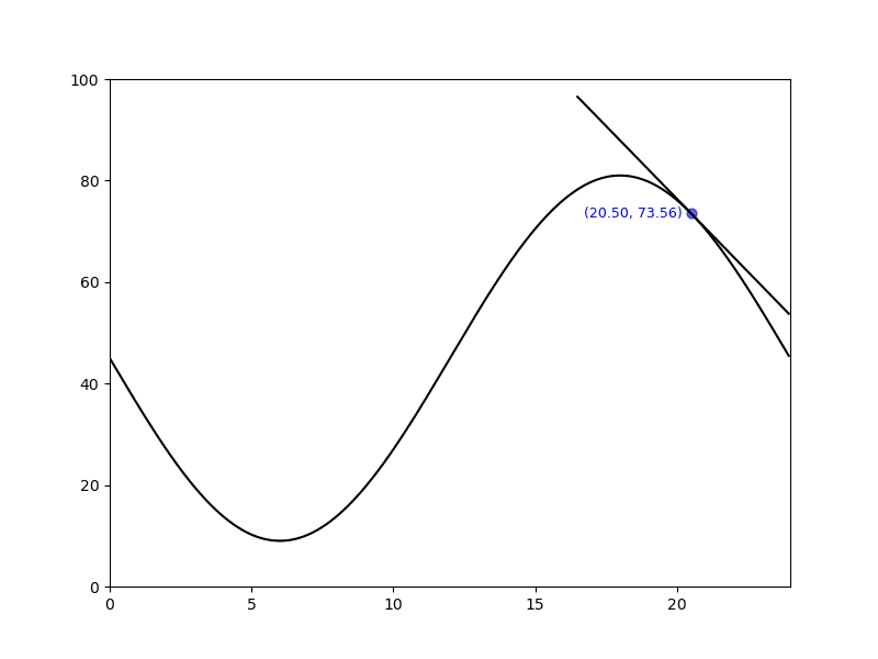
Looks like the function works as intended. I know, not thorough testing, but…
Time to move on to the last bit—placing the text (equation for tangent) in a suitable location on the plot axis.
draw_tangent_text()
As mentioned above this function will do some calculations, draw the tangent on the plot axis using the function above, then figure out where to put the text of the tangent’s equation. Once it has that it will draw the text and return.
Full function code below. Did remove one parameter shown in the design note above.
I will let you sort how I got to the code. Pretty simple approach. Too much code? Another helper function?
def draw_tangent_txt(ax, px1, py1, slp, t_font):
  ''' Calculate the point at which to place tangent equation text.
      Plot tangent and draw text to supplied figure axis.

  :param ax: matplotlib plot axes
  :param px1: x-axis value for point of interest
  :param py1: y-axis value for point of interest
  :param slp: differential for (tx1, ty1), i.e. slope of tangent line
  :param p_font: initial font dict to use for point related text
                 keys expected: 'color', 'size', 'va'
                 'color' and 'size' values will not change,
                 'ha' may be added, and 'va' changed

  Side effect: draws dot and text at data point location
  Returns: nothing
  '''
  # process debug related code

  # we could use ax.get_window_extent to determine these values, but...
  # x_min, x_max = 0, 24
  # at this point should only be one Line2D object on the plot,
  #  the state of charge curve
  if len(ax.lines) == 1:
    soc_bbx = get_artist_bbox(ax.lines[0])
    x_mn, x_mx, y_mn, y_mx = soc_bbx.x0, soc_bbx.x1, soc_bbx.y0, soc_bbx.y1

  x_sep = .4
  is_ok = False
  f_txt = copy.deepcopy(t_font)

  t_str, t_fn, t_inv, t_bbx = draw_tangent(ax, px1, py1, slp, f_txt)

  # code to sort text position and draw text to passed axis
  # if tangent extends below or above soc curve put text between
  #   curve axis min/max and end of tangent line as appropriate
  if t_bbx.y0 < soc_bbx.y0:
    # below curve minimum
    f_txt["ha"] = "left"
    t_btm = max(t_bbx.y0, 0)
    y_txt = soc_bbx.y0 - ((soc_bbx.y0 - t_btm) / 2)
    x_txt = t_inv(y_txt) + x_sep
    ax.text(x_txt, y_txt, t_str, fontdict=f_txt)
  elif t_bbx.y1 > soc_bbx.y1:
    # above curve maximum
    f_txt["ha"] = "right"
    t_top = min(t_bbx.y1, 100)
    y_txt = soc_bbx.y1 + ((t_top - soc_bbx.y1) / 2)
    x_txt = t_inv(y_txt) - x_sep
    ax.text(x_txt, y_txt, t_str, fontdict=f_txt)
  # otherwise put code ??
  else:
    # don't think this is actually necessary for our curve
    # with the default length of the tangent line, it always
    # seems to end above curve maximum or below minimum
    f_txt["ha"] = "right"
    t_top = min(t_bbx.y1, 100)
    y_txt = soc_bbx.y1 + ((t_top - soc_bbx.y1) / 2)
    x_txt = t_inv(y_txt) - x_sep
    ax.text(x_txt, y_txt, t_str, fontdict=f_txt)
I am going to write some test code that will plot, twice, three different points to the chart. Don’t want a pile of images added to the post. A couple plots with three points each should be enough. And, not going to bother including the test code.
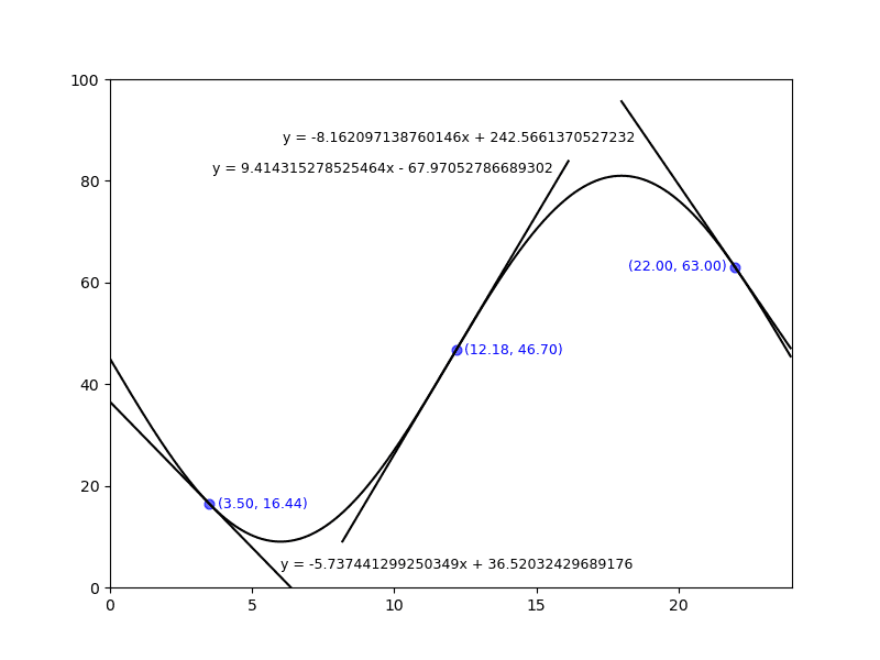
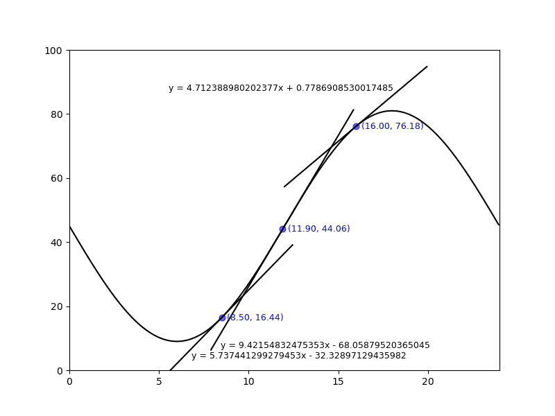
And, there you go. Not perfect, but seems to work. And no hardcoded positions needed to draw the text!
Done!!
I think that’s finally it for this wee road trip off the beaten path. Not sure it was truly of value. But, I did learn a great deal more about plotting with matplotlib than I ever imagined I would. And likely not the last such adventure.
May your side trips be shorter and more scenic than this last one of mine.
Resources
- Under the hood of matplotlib